A short example of ctaplot functions

import ctaplot
import numpy as np
import matplotlib.pyplot as plt
import astropy.units as u

ctaplot.set_style('slides')

Generate some dummy data

size = 1000
simu_energy = 10**np.random.uniform(-2, 2, size) * u.TeV
reco_energy = simu_energy.value**0.9 * simu_energy.unit
source_alt = 3. * u.rad
source_az = 1.5 * u.rad
simu_alt = source_alt * np.ones(size)
simu_az = source_az * np.ones(size)
reco_alt = np.random.normal(loc=source_alt.to_value(u.rad), scale=2e-3, size=size) * u.rad
reco_az = np.random.normal(loc=source_az.to_value(u.rad)-0.005, scale=2e-3, size=size) * u.rad

Position reconstruction

# ctaplot.plot_field_of_view_map(reco_alt, reco_az, source_alt, source_az);

fig, axes = plt.subplots(1, 2, figsize=(20,5))
ctaplot.plot_theta2(reco_alt, reco_az, simu_alt, simu_az, bins=40, ax=axes[0])
ctaplot.plot_angular_resolution_per_energy(reco_alt, reco_az, simu_alt, simu_az, simu_energy, ax=axes[1])
ctaplot.plot_angular_resolution_cta_requirement('south', ax=axes[1], color='black')
axes[1].legend();
plt.show()

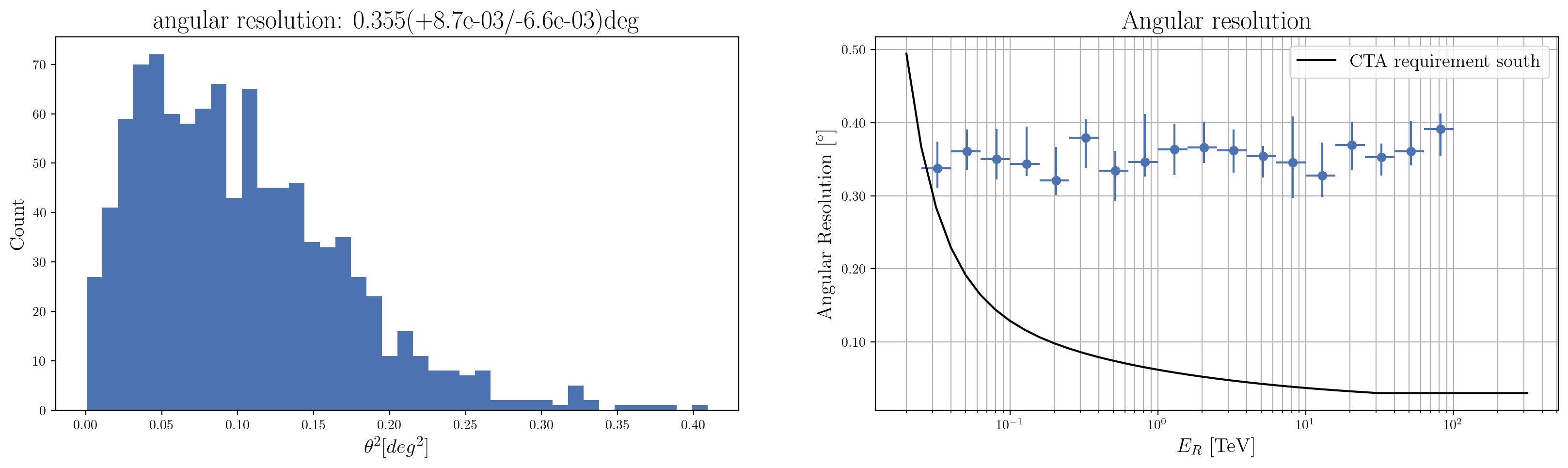
Ok, the position is really not well reconstructed.

But this is actually because of a bias in the reconstruction. We can ask for an automatic correction of this bias.

fig, axes = plt.subplots(1, 2, figsize=(20,5))
ctaplot.plot_theta2(reco_alt, reco_az, simu_alt, simu_az,
                    bins=40,
                    bias_correction=True,
                    ax=axes[0])

ctaplot.plot_angular_resolution_per_energy(reco_alt, reco_az, simu_alt, simu_az, simu_energy,
                                           bias_correction=True,
                                           ax=axes[1])

ctaplot.plot_angular_resolution_cta_requirement('south', ax=axes[1], color='black')
axes[1].legend()
plt.show()

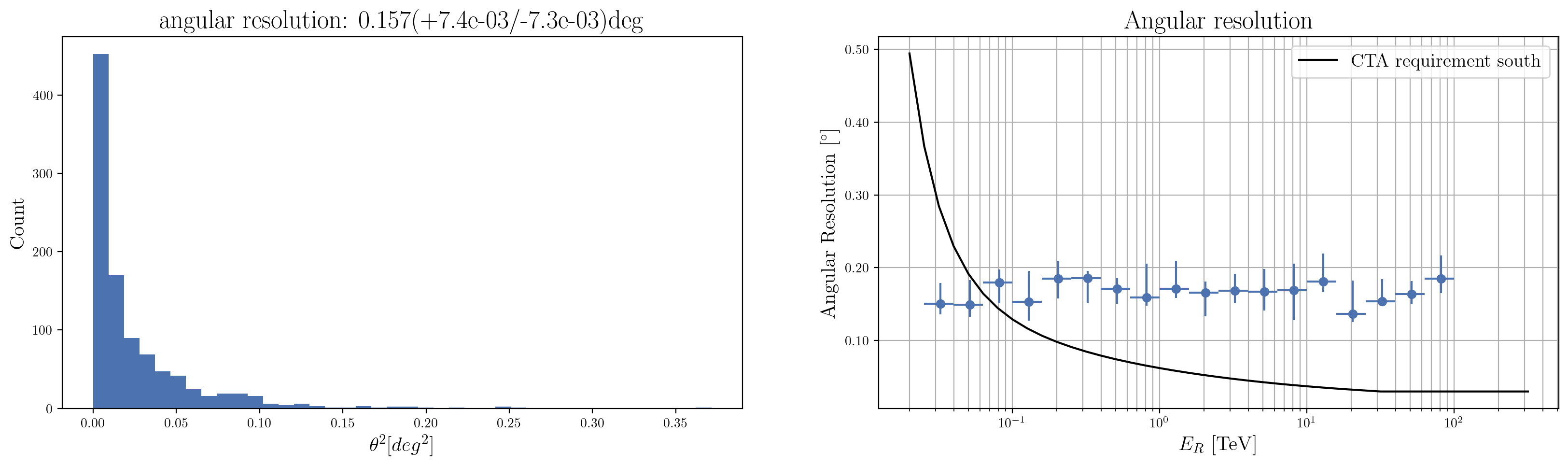
Now the angular resolution looks better, in agreement with the input scale of the Gaussian distribution.

Energy reconstruction

plt.figure(figsize=(12,7))
ax = ctaplot.plot_energy_resolution(simu_energy, reco_energy)
ctaplot.plot_energy_resolution_cta_requirement('north', ax=ax)
ax.legend()
plt.show()

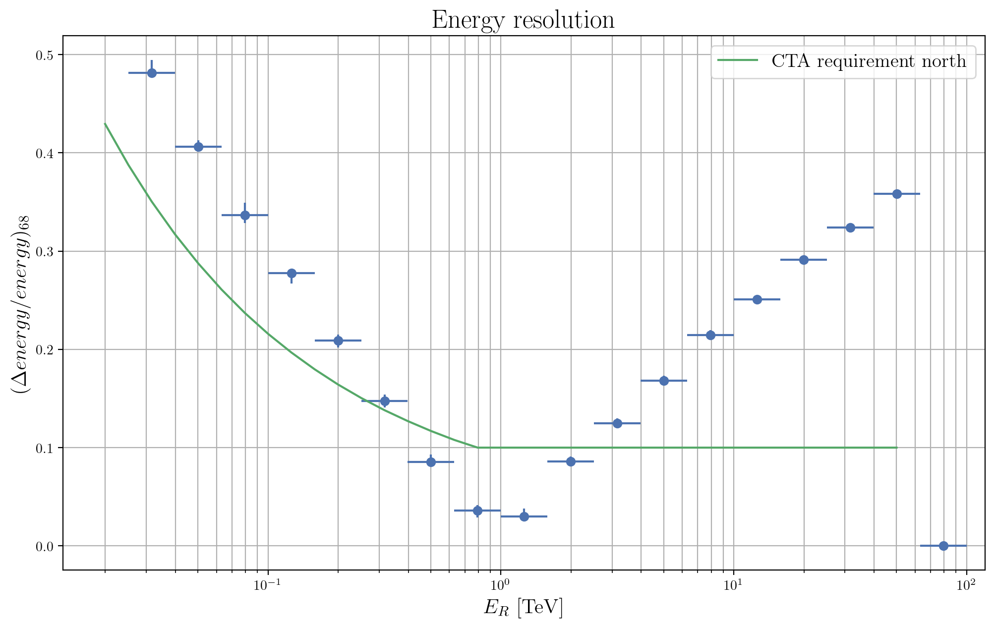
But you might want to study the energy resolution as a function of another variable… or to compute the resolution of other stuff

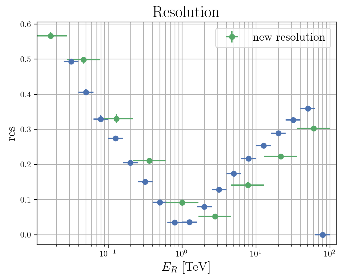
new_variable = simu_energy * 2

bins, res = ctaplot.resolution_per_bin(new_variable, simu_energy, reco_energy,
                                       bins=np.logspace(-2,2,10)*u.TeV,
                                       relative_scaling_method='s1')

ax = ctaplot.plot_energy_resolution(simu_energy, reco_energy)
ctaplot.plot_resolution(bins, res, label='new resolution', ax=ax, log=True)
ax.legend()
plt.show()